Regression Discontinuity in R
By Josh McCrain
 Twitter
1 Introduction
Regression discontinuity is a common identification strategy in the Congress literature. There are lots of elections and many close elections providing enough power for estimating local average treatment effects. However, there are numerous tools and approaches to actually visualizing these relationships, estimating the regressions, and calculating bandwidths.
In this separate section of the guide I’ll cover how you can prepare your data to make these plots, and then how to use the rdrobust package to estimate bandwidth-optimal regression discontinuities. I also show how to easily visualize the discontinuity using ggplot2.
I won’t get into the statistics behind what’s going on; this is meant to be a resource for how to navigate this task using R and the tidyverse tools.
2 Preparing the data
For this example I’m going to use elections data compiled from CQ. Unfortunately you have to have a subscription to CQ to access these data (most academics will have one), so I can’t share the dataset publicly. However, this process will be the same for any dataset that has election returns.
Importantly, as you’ll see, you need full election returns data, not just the voteshare of the winning candidate.
First, load in the data.
##  [1] "state"   "year"    "office"  "dist"    "name_D"  "party_D" "vote_D"
##  [8] "inc_D"   "name_R"  "party_R" "vote_R"  "inc_R"   "name_D2" "vote_D2"
## [15] "inc_D2"  "name_R2" "vote_R2" "inc_R2"  "type"    "nextup"  "race"
## [22] "name_O"  "party_O" "vote_O"  "inc_O"
This is a very basic panel dataset of one observation per election year (including special elections). What we want out of this is the votemargin of the winning candidate. Or, another way of approaching this problem substantively is to think about what happens to a district if that district is randomly assigned a Democrat versus a Republican member of Congress.
With an RD, we can approximate this randomization using close elections. So what we need specifically is the how much the winning candidate won by in vote percentage. If we just had their total voteshare, this might omit 3rd party votes. For instance, if the winning candidate received 55% of the vote but the second place candidate received 40%, the winner won by 15% instead of 10%.
Let’s grab that from the data while subsetting the data to only open seat elections:
house_full$inc_O[is.na(house_full$inc_O)] <- 0

house_rd <- house_full %>%
  filter(inc_D == 0 & inc_R == 0 & inc_O == 0) %>% # only open seat elections
  mutate(vote_O = ifelse(is.na(vote_O), 0, vote_O)) %>%
  mutate(total_vote = vote_D + vote_R + vote_O,
         perc_R = vote_R / total_vote) %>%
  select(state, year, dist, vote_D, vote_R, vote_O, total_vote, perc_R)

head(house_rd)
## state year dist vote_D vote_R vote_O total_vote perc_R
## 1 AK 1973 1 33123 35044 0 68167 0.5140904
## 2 AL 1980 6 87536 95019 3218 185773 0.5114791
## 3 AL 1984 1 98455 102479 0 200934 0.5100132
## 4 AL 1986 7 108126 72777 0 180903 0.4022985
## 5 AL 1989 3 47294 25142 0 72436 0.3470926
## 6 AL 1990 5 113047 55326 0 168373 0.3285919As with most RD applications, your sample will be quite small from the start and will only get smaller as you’ll only use observations close to the cutoff (here the cutoff is 50%).
##     state                year           dist            vote_D
##  Length:647         Min.   :1972   Min.   : 1.000   Min.   :  3514
##  Class :character   1st Qu.:1980   1st Qu.: 2.000   1st Qu.: 70534
##  Mode  :character   Median :1992   Median : 5.000   Median : 90926
##                     Mean   :1992   Mean   : 8.935   Mean   : 94937
##                     3rd Qu.:2002   3rd Qu.:12.000   3rd Qu.:114645
##                     Max.   :2016   Max.   :52.000   Max.   :233554
##      vote_R           vote_O        total_vote         perc_R
##  Min.   :  7959   Min.   :    0   Min.   : 13753   Min.   :0.4020
##  1st Qu.: 74945   1st Qu.:    0   1st Qu.:149394   1st Qu.:0.4621
##  Median : 96524   Median :    0   Median :191508   Median :0.5038
##  Mean   :100083   Mean   : 3478   Mean   :198498   Mean   :0.5031
##  3rd Qu.:123130   3rd Qu.: 4346   3rd Qu.:237951   3rd Qu.:0.5467
##  Max.   :255468   Max.   :90026   Max.   :460407   Max.   :0.5999
Now we’ll read in some data for covariates and outcomes. This is data I’ve used elsewhere in the guide from the Historical Congressional Legislation and District Demographics dataverse repository. We’ll read this in and drop elections after the 111th Congress to match our other data.
Next, let’s read in some district spending replication data, also used elsewhere: Distributive Politics and Legislator Ideology Replication Data
I’m going to clean this up as discussed in Working with Messy Data. The idea is that I want to merge it together with the other data of interest and use the ln_grants_nf variable as an outcome in the regression.
library(readstata13)

abh <- read.dta13("data/ABH_full_district.dta")
abh <- select(abh, year, cong = congress, dist, fips_state, ln_grants_nf, ln_grants_all)
abh <- abh %>%
  ungroup %>%
  group_by(fips_state, cong, dist) %>%
  summarize_at(vars(ln_grants_nf, ln_grants_all), mean)

abh <- abh %>%
  ungroup %>%
  mutate(fips_state = parse_number(fips_state))

library(maps) # for state.fips data

abh <- state.fips %>%
  select(fips_state = fips, state = abb) %>%
  group_by(fips_state) %>%
  distinct(state) %>%
  left_join(abh, .)
We now have our datasets almost ready to merge. However, the elections data is at the year level but our other data are at the Congress level. Let’s add in years:
cong.years <- data.frame(year = seq(1971, 2009),
                         cong = c(92, rep(seq(93, 111), each=2)))

house_rd <- left_join(house_rd, cong.years) %>%
  filter(!is.na(cong))
## Joining, by = "year"Now we can put it all together. This step all cleans the RD panel by dropping special elections, a substantive choice I’m making since I want to make apples-to-apples comparisons.
This step also creates logged versions of a couple variables we can use later in the analysis.
## Joining, by = c("state", "dist", "cong")house_rd <- cong_data %>%
group_by(state, cd, congNum) %>%
arrange(numberTerms) %>%
filter(row_number()==1) %>%
ungroup %>%
select(state, dist = cd, cong = congNum, prcntBA, gender, numSpon, numCosp) %>%
mutate(log_numSpon = log(numSpon + 1),
log_numCosp = log(numCosp + 1)) %>%
left_join(house_rd, .)## Joining, by = c("state", "dist", "cong")3 Visualization
I find that visualizing the discontinuity of interest is a good first step. However, you should note that these visualizations do not necessarily tell us much about the statistical significance of the treatment effect at the cutoff. For that we’ll run some regressions, which are below.
house_rd %>%
  ungroup %>%
  mutate(`Party Won` = ifelse(perc_R < .5, "Democrat", "Republican")) %>%
  filter(!is.na(`Party Won`)) %>%
  filter(perc_R >= .4 & perc_R <= .6) %>%
  ggplot(aes(x = perc_R, y = ln_grants_nf, group=`Party Won`, color=`Party Won`)) +
  geom_point() +
  geom_smooth(method="lm") +
  ylim(14, 22)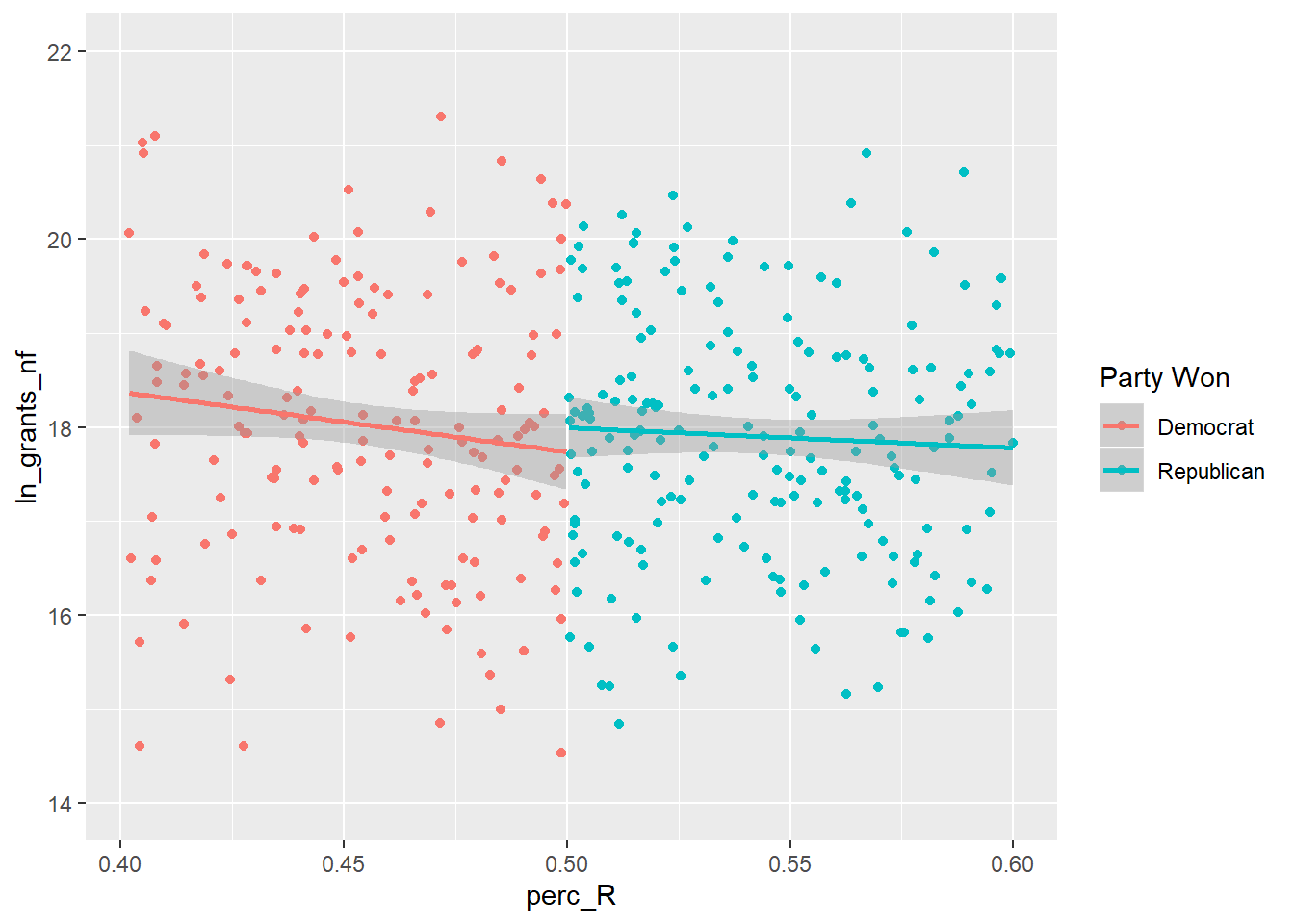
The key to this visualization is dividing the observations in groups based on which side of the cutoff they fall on. I create the new variable Party Won to do this, and then pass that as the grouping and color variable to ggplot.
I then plot the individual observations with geom_point and have ggplot plot a basic OLS line, plotted separately on each side of the cutoff, using geom_smooth (you can change this to a higher order polynomial if desired).
The “forcing” or “running” variable on the x-axis is the Republican vote share and the outcome variable is the grants received by that district.
Let’s do the same using the number of sponsors that member received on bills as the outcome:
house_rd %>%
  ungroup %>%
  mutate(`Party Won` = ifelse(perc_R < .5, "Democrat", "Republican")) %>%
  filter(!is.na(`Party Won`)) %>%
  filter(perc_R >= .4 & perc_R <= .6) %>%
  ggplot(aes(x = perc_R, y = log_numSpon, group=`Party Won`, color=`Party Won`)) +
  geom_point() +
geom_smooth(method="lm") 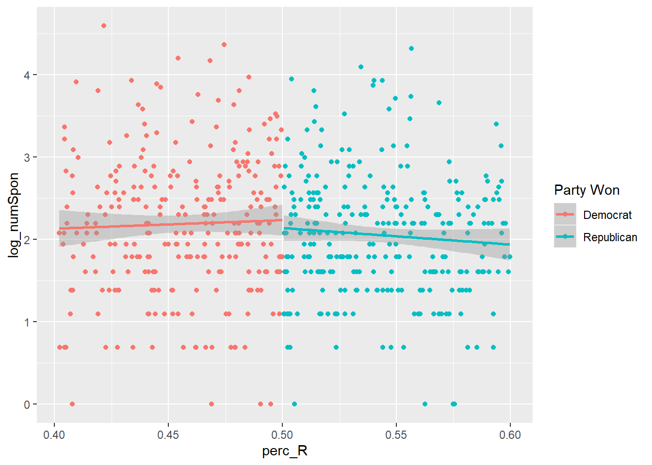
Both of these plots show a little action around the cutoff, but they’re a bit messy and it’s not obvious if it’s statistically significant. Let’s clean up the figure first:
I like replacing the big clouds of points with points summarizing local averages. This is actually pretty easy to do:
points <- house_rd %>%
  ungroup %>%
  filter(perc_R >= .4 & perc_R <= .6) %>%
  mutate(perc_R = round(perc_R, 3)) %>%
  group_by(perc_R) %>%
  summarize(log_numSpon = mean(log_numSpon),
            num_obs = n())

house_rd %>%
  ungroup %>%
  mutate(`Party Won` = ifelse(perc_R < .5, "Democrat", "Republican")) %>%
  filter(!is.na(`Party Won`)) %>%
  filter(perc_R >= .4 & perc_R <= .6) %>%
  ggplot(aes(x = perc_R, y = log_numSpon, group=`Party Won`, color=`Party Won`)) +
  geom_point(data = points, aes(x = perc_R, y=log_numSpon, size=num_obs), alpha=.2, inherit.aes=F) +
geom_smooth(method="lm") 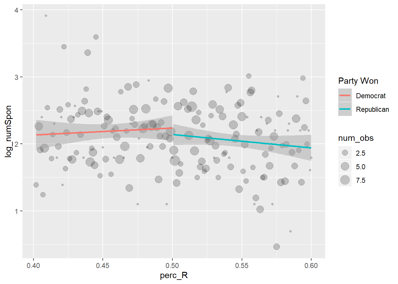
Essentially what is happening to create the points dataframe is I’m binning the observations together by the rounded Republican vote share. Then, I summarize based on the rounded vote share to get the mean value of sponsorship (or local average) and the total number of observations at that location. The total number of observations – total_obs is then used in ggplot to weight the size of each point.
You can also do this all in one long piping procedure if you want to be really cool. We’ll also clean the graph up a bit:
house_rd %>%
  ungroup %>%
  mutate(`Party Won` = ifelse(perc_R < .5, "Democrat", "Republican")) %>%
  filter(!is.na(`Party Won`)) %>%
  filter(perc_R >= .4 & perc_R <= .6) %>%
  ggplot(aes(x = perc_R, y = ln_grants_nf, group=`Party Won`, color=`Party Won`)) +
  geom_point(data= house_rd %>%
              ungroup %>%
              filter(perc_R >= .4 & perc_R <= .6) %>%
              mutate(perc_R = round(perc_R, 3)) %>%
              group_by(perc_R) %>%
              summarize(ln_grants_nf = mean(ln_grants_nf),
                        num_obs = n()),
             aes(x = perc_R, y=ln_grants_nf, size=num_obs), alpha=.2, inherit.aes=F) +
  geom_smooth(method="lm") +
  scale_color_manual(values=c("dodgerblue", "red4")) +
  geom_vline(xintercept=.5, linetype="dashed", alpha=.7) +
  theme_classic() +
  xlab("Republican Voteshare") + ylab("District Grants (logged)")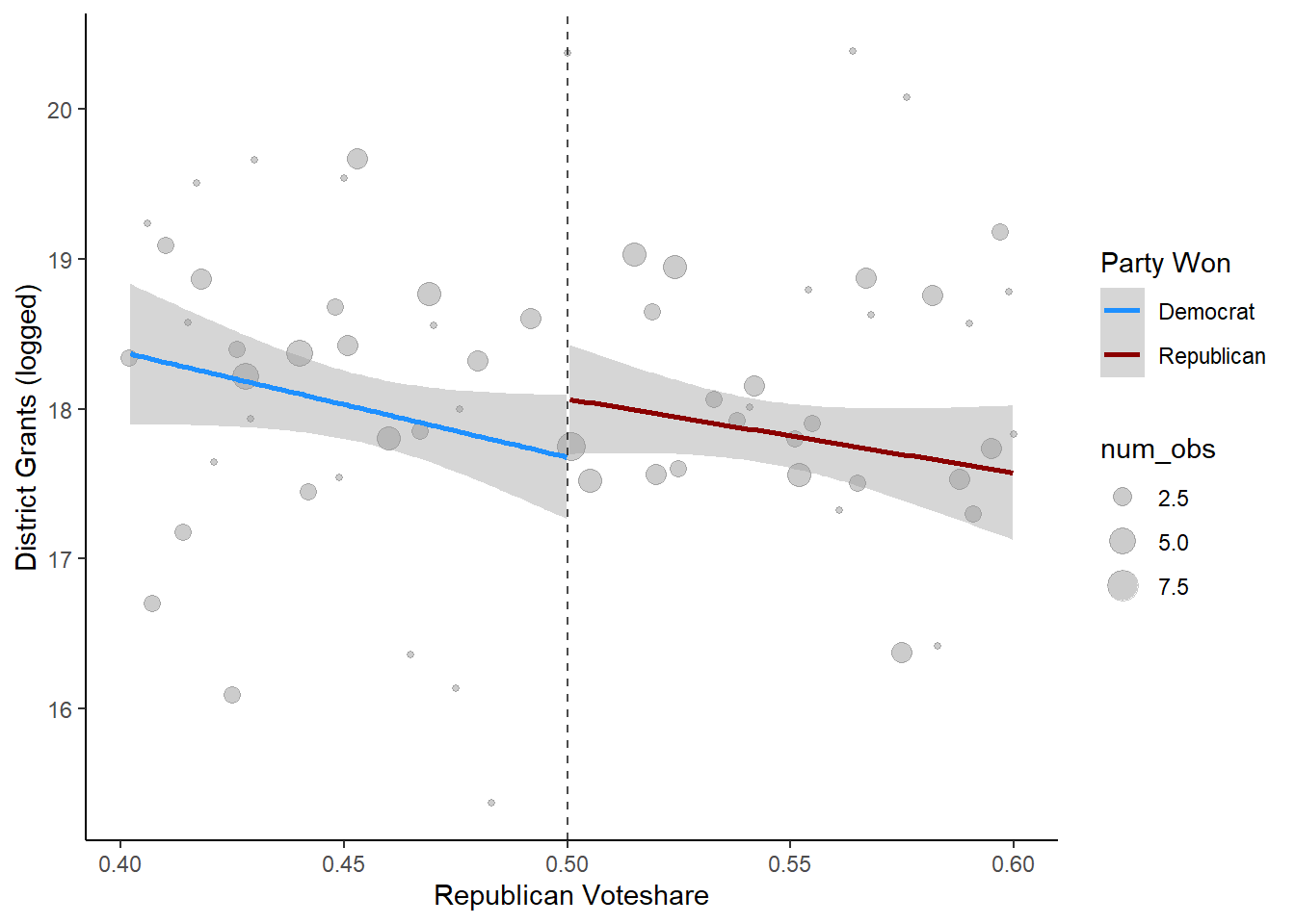
Again, it looks like there might be something there but it’s pretty close. It’s possible that districts that see Republicans narrowly win instead of narrowly lose get more money in the subsequent congress. We need to turn to actual regressions to find out:
4 Regression Discontinuity
Again, I’m not going to go through the nuts and bolts of why we’re doing all of this from a statistics point of view. This is simply how to use your data in R to run thse kinds of regressions.
First, let’s create a few useful variables:
rep_won- a dummy variable if the Republican won the electionvotemargin- how much above or below 50% of the vote did the candidate receivef_x_win- an interaction between these two variablesstateDist- a state district fixed effect
house_rd$rep_won <- NA
house_rd$rep_won[house_rd$perc_R > .5] <- 1
house_rd$rep_won[house_rd$perc_R < .5] <- 0

house_rd$votemargin <- house_rd$perc_R - .5

house_rd$f_x_win <- house_rd$votemargin * house_rd$rep_won

house_rd <- house_rd %>%
  ungroup %>%
  mutate(stateDist = paste(state, dist, sep="."))
4.1 Bandwidth selection
Now we’re going to use the rdrobust package and the rdbwselect function to determine the optimal bandwidth size. This is very important and this package makes it easy. I am also adding covariates to the bandwidth selection using the function’s covs argument.
library(rdrobust)

grants_rd <- house_rd %>%
  filter(!is.na(ln_grants_nf))

grants_rd$cutoff<-NULL
grants_rd$bandwidth<-NULL
grants_rd$kw<-NULL

bws <- rdbwselect(grants_rd$ln_grants_nf, grants_rd$votemargin, p=1, c = 0,
                  kernel = "tri", bwselect="mserd",
                  covs = grants_rd$prcntBA + grants_rd$year)

grants_rd$bandwidth <- bws$bws[1]

grants_rd$cutoff <- 0

grants_rd$kw <- 1-(abs(grants_rd$cutoff - grants_rd$votemargin))/grants_rd$bandwidth

grants_rd$kw[grants_rd$votemargin > (grants_rd$cutoff + grants_rd$bandwidth) |
               grants_rd$votemargin < (grants_rd$cutoff - grants_rd$bandwidth)] <- 0
After the rdbwselect function finds the optimal bandwidth, I assign that value to a new column in my data. I then create the kernel weight, kw, using the bandwidth, votemargin and cutoff.
4.2 Estimation
We’re now ready to run regressions. The lfe package works great here since it makes dealing with fixed effects, clustering, and weighting easy. Let’s run two models, one with controls and one without.
model1 <- felm(grants_rd$ln_grants_nf[grants_rd$kw > 0] ~ votemargin + rep_won + f_x_win  |
                year | 0 | stateDist, data = grants_rd[grants_rd$kw > 0, ], weights = grants_rd$kw[grants_rd$kw > 0])

model2 <- felm(grants_rd$ln_grants_nf[grants_rd$kw > 0] ~ votemargin + rep_won + f_x_win + prcntBA | year
              | 0 | stateDist, data = grants_rd[grants_rd$kw > 0, ], weights = grants_rd$kw[grants_rd$kw > 0])

summary(model1)
##
## Call:
## felm(formula = grants_rd$ln_grants_nf[grants_rd$kw > 0] ~ votemargin + rep_won + f_x_win | year | 0 | stateDist, data = grants_rd[grants_rd$kw > 0, ], weights = grants_rd$kw[grants_rd$kw > 0])
##
## Weighted Residuals:
## Min 1Q Median 3Q Max
## -2.70688 -0.47355 -0.07125 0.44493 2.64916
##
## Coefficients:
## Estimate Cluster s.e. t value Pr(>|t|)
## votemargin 6.369e+00 8.635e+00 0.738 0.462
## rep_won -8.922e-05 2.894e-01 0.000 1.000
## f_x_win -5.394e+00 1.194e+01 -0.452 0.652
##
## Residual standard error: 0.7898 on 217 degrees of freedom
## Multiple R-squared(full model): 0.5179 Adjusted R-squared: 0.4713
## Multiple R-squared(proj model): 0.006984 Adjusted R-squared: -0.08911
## F-statistic(full model, *iid*): 11.1 on 21 and 217 DF, p-value: < 2.2e-16
## F-statistic(proj model): 0.5828 on 3 and 188 DF, p-value: 0.627##
## Call:
## felm(formula = grants_rd$ln_grants_nf[grants_rd$kw > 0] ~ votemargin + rep_won + f_x_win + prcntBA | year | 0 | stateDist, data = grants_rd[grants_rd$kw > 0, ], weights = grants_rd$kw[grants_rd$kw > 0])
##
## Weighted Residuals:
## Min 1Q Median 3Q Max
## -2.62208 -0.49352 -0.06607 0.44485 2.43438
##
## Coefficients:
## Estimate Cluster s.e. t value Pr(>|t|)
## votemargin 5.88228 8.62186 0.682 0.49581
## rep_won -0.08746 0.29631 -0.295 0.76814
## f_x_win -2.95059 12.14255 -0.243 0.80824
## prcntBA 0.02974 0.01019 2.920 0.00388 **
## ---
## Signif. codes: 0 '***' 0.001 '**' 0.01 '*' 0.05 '.' 0.1 ' ' 1
##
## Residual standard error: 0.771 on 216 degrees of freedom
## Multiple R-squared(full model): 0.5427 Adjusted R-squared: 0.4962
## Multiple R-squared(proj model): 0.05812 Adjusted R-squared: -0.03781
## F-statistic(full model, *iid*):11.65 on 22 and 216 DF, p-value: < 2.2e-16
## F-statistic(proj model): 2.783 on 4 and 188 DF, p-value: 0.02803In both models there does not appear to be any statistical significance in the relationship between Republicans winning close elections and grants to a district.
Let’s try the sponsorship variable as the outcome now. We’re doing the exact same thing as above.
spon_rd <- house_rd %>%
  filter(!is.na(log_numSpon) & !is.na(perc_R))

spon_rd$cutoff<-NULL
spon_rd$bandwidth<-NULL
spon_rd$kw<-NULL

bws <- rdbwselect(spon_rd$log_numSpon, spon_rd$votemargin, p=1, c = 0,
                  kernel = "tri", bwselect="mserd",
                  covs = spon_rd$prcntBA + spon_rd$year)

spon_rd$bandwidth <- bws$bws[1]

spon_rd$cutoff <- 0

spon_rd$kw <- 1-(abs(spon_rd$cutoff - spon_rd$votemargin))/spon_rd$bandwidth

spon_rd$kw[spon_rd$votemargin > (spon_rd$cutoff + spon_rd$bandwidth) |
               spon_rd$votemargin < (spon_rd$cutoff - spon_rd$bandwidth)] <- 0

# run the same model
model2 <- felm(spon_rd$log_numSpon[spon_rd$kw > 0] ~ votemargin + rep_won + f_x_win + prcntBA | year
              | 0 | stateDist, data = spon_rd[spon_rd$kw > 0, ], weights = spon_rd$kw[spon_rd$kw > 0])


summary(model2)
##
## Call:
## felm(formula = spon_rd$log_numSpon[spon_rd$kw > 0] ~ votemargin + rep_won + f_x_win + prcntBA | year | 0 | stateDist, data = spon_rd[spon_rd$kw > 0, ], weights = spon_rd$kw[spon_rd$kw > 0])
##
## Weighted Residuals:
## Min 1Q Median 3Q Max
## -1.84626 -0.23958 0.01435 0.25891 1.64032
##
## Coefficients:
## Estimate Cluster s.e. t value Pr(>|t|)
## votemargin 3.210817 3.505341 0.916 0.360249
## rep_won -0.237257 0.144848 -1.638 0.102241
## f_x_win -1.105898 4.415133 -0.250 0.802350
## prcntBA 0.018854 0.005344 3.528 0.000469 ***
## ---
## Signif. codes: 0 '***' 0.001 '**' 0.01 '*' 0.05 '.' 0.1 ' ' 1
##
## Residual standard error: 0.4917 on 387 degrees of freedom
## Multiple R-squared(full model): 0.3479 Adjusted R-squared: 0.2923
## Multiple R-squared(proj model): 0.04655 Adjusted R-squared: -0.03475
## F-statistic(full model, *iid*):6.256 on 33 and 387 DF, p-value: < 2.2e-16
## F-statistic(proj model): 4.298 on 4 and 270 DF, p-value: 0.002182Again, there is no statistical significance. While the figures above were suggestive of a possible relationship, once we use optimal bandwidth selection and controls the relationship disappears. These model objects are easy to work with and you can use all of the same tools for visualization as I covered previously.